Walking Through a Linear Regression

A full breakdown of the machine learning process

A linear regression serves as the cornerstone algorithm when working with data. It is widely used and one of the most applicable supervised machine learning algorithms in existence. By performing linear regression, we are trying to capture the best linear relationship between predicting independent variables (X1, X2, etc…) and a predicted dependent variable (Y). Together, let’s walk through a linear regression model process in Python. The repository, with all code and data, can be found here.

The Set-Up

We will be using a simulated dataset representing carseat sales for a company. The company wants for their data team to put together a model which will accurately capture and predict their carseat sales movements for their store locations, given a dataset with a number of predicting independent variables. The variable descriptions are as follows:

Sales: unit sales at each location
CompPrice: price charged by the nearest competitor at each location
Income: community income level
Advertising: local advertising budget for the company at each location
Population: population size in the region (in thousands)
Price: price charged for a car seat at each site
ShelveLoc: quality of shelving location at site (Good | Bad | Medium)
Age: average age of the local population
Education: education level at each location
Urban: whether the store is in an urban or rural location
USA: whether the store is in the US or not

Sales will be our dependent variable (or target) and the remaining 10 variables (features) will be processed and manipulated to assist in our regression. It is important to note at this point what our variables consist of. We have certain variables, such as income, advertising, or population which are all integer based variables. However, we also have variables like Urban, USA, and ShelveLoc. The values for these variables are representing categorical values (Yes/No; Good/Bad/Medium; etc.). We will see how to account for these differences as we progress, it is just important to note at this stage that they are different. (Utilizing the ‘df.info()’ command in Python will assist in identifying the makeup of your variable values.

Here is a snapshot of our DataFrame:

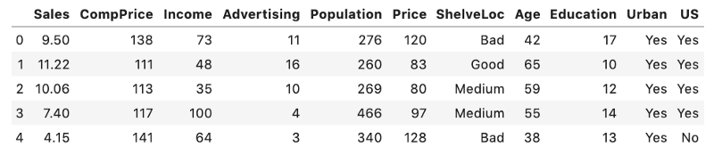
df.head()

Pre-processing

The pre-processing stage is, shockingly, where we prepare our DataFrame and its contents before building the model. In this phase, we will perform a train-test-split, deal with the categorical variables mentioned above using encoding, and finally take care of any scaling issues which may be present.

The first thing we need to do is separate our DataFrame into our target series and predictor series. X will be our DataFrame of independent variables while y will be our target feature.

X = df.drop('Sales', axis = 1)
y = df.Sales

Now that we have each split, we can perform the train-test-split. This step is vital to our machine learning model. We split our data into a ‘train’ and a ‘test’ group. The train set will be used for our model to actually learn from, and our test set will be used to as validation for the output, being that we already know those values. In order for us to access this feature, we must import it from Sklearn. We have 400 data entries, which is a decently sufficient data size, so we will use a 70/30 percent ratio for our train size and test size, respectively (for our test_size argument in the function).

from sklearn.preprocessing import train_test_split

X_train, X_test, y_train, y_test = train_test_split(X, y, test_size = .30, random_state = 33)

Next, we need to conduct some quick cleaning procedures. Let’s remove any duplicate values or missing values from our training dataset.

X_train.drop_duplicates(inplace = True)
X_train.dropna(inplace = True)

Dealing with Different Data Types

As we mentioned earlier, it is essential that we differentiate the types of data in our set. This requires us to separate numerical data (integers or continuous numbers) from categorical data (binary outcomes, locations represented by numbers, etc.). At this point, all data types are included in our X_train.

X_train.info()

We see the data types in the third column where all features, except for three, have data type ‘int64’, meaning that our DataFrame is interpreting that data as integers. These will be treated as our numeric data. The remaining three, the categorical variables, will be temporarily excluded.

Numeric Data

The code block below will select features with all datatypes excluding ‘object’, our categorical data. The second and third lines of code just bring over column titles from our X_train.

X_train_numerics = X_train.select_dtypes(exclude = 'object')
X_train_cols = X_train.columns
X_train_numerics.columns = X_train_cols

Just to verify, below on the left is the data information of our new, numeric-type-only dataset. The figure below on the right is a snapshot of what our numeric DataFrame actually looks like.

Even though we have all of our numeric data now together, our pre-processing work is not complete. Now we must understand what each numeric series contains. For example, ‘CompPrice’ represents a dollar figure from another competitor, however ‘Education’ represents an education level at each location but we don’t have any further information. Population represents (in thousands) how many people are in a respective area. Even though these are all forms of numeric data, we can’t really compare them because the units are all different! How do we deal with this conundrum? Scaling!

Scaling our Data

Scaling will allow for all of our data to be transformed into a more normal distribution. We will be using the StandardScaler method from Sklearn. This function will effectively standardize respective features by removing the mean and scaling to unit variance. This function will allow for us to remove any effects that would be present from having one feature (say CompPrice, due to its larger values) from having an incorrect magnitude of influence on our predictor variable.

from sklearn.preprocessing import StandardScaler
from scipy import stats

ss = StandardScaler()

X_train_numeric = pd.DataFrame(ss.fit_transform(X_train_numeric))
X_train_numeric.set_index(X_train.index, inplace = True)

X_train_numeric.columns = X_numeric_cols
X_train_numeric.head()

First, we import and instantiate a StandardScaler object. We then fit and transform our numeric DataFrame and set the index feature equal to that of our original X_train. This will ensure we are operating on the correct data entries. We must set the column names once again because they were removed when passing through the StandardScaler object. Our resulting data looks like this:

We notice a couple of things. Our data values no longer resembles what it did before. We have removed any and all magnitude differentiation of our original features and they are now all on a unanimous scale, without any individual feature having an inaccurate influence over our predicting variable.

Removing Outliers

Our last step when working with our numeric data is to remove any outliers. Outliers can cause an inaccurate representation of feature data as a small number of entry values can have inaccurate influences on another variable. We will do this by using the ‘stats’ package and filtering any values with a z-score value greater than 2.5 standard deviations away from the mean.

X_train_numeric = X_train_numeric[(np.abs(stats.zscore(X_train_numeric)) < 2.5).all(axis = 1)]

Categorical Data

Now that we’ve taken care of preparing our numeric data, we want to address our categorical data. Let’s isolate our categorical data into its own DataFrame and take a look at what we’re working with. This is the same first step as when working with numeric, we just change the argument inside of our ‘select_dtypes’ method from ‘exclude’ to ‘include’.

X_train_cat = X_train.select_dtypes(include = 'object')

The right figure shows us what our categorical DataFrame actually looks at. It would be pretty cool if our computers could figure out how to interpret ‘Good’, ‘Medium’, or ‘Yes’, but unfortunately, it is not that smart yet — we will save the NLP models for later ;). At this point, we need to convert these values into something our computer can understand via a process called encoding.

Encoding Categorical Data

Let’s begin dealing with our Urban and US variables. These variables are both binary (“yes” or “no”) so we want to express these as binary values to our computer instead of as “yes” or “no”. We will use sklearn’s LabelBinarizer function to do so. To use the function, we first instantiate a LabelBinarizer() object for each respective feature, and then perform a fit_transform on each.

from sklearn.preprocessing import LabelBinarizer

urban_bin = LabelBinarizer()
us_bin = LabelBinarizer()

X_train_cat.Urban = urban_bin.fit_transform(X_train_cat.Urban)
X_train_cat.US = us_bin.fit_transform(X_train_cat.US)

Our resulting DataFrame now represents ‘Yes’ as a 1 and ‘No’ as a 0. Now let’s turn our attention to the ‘ShelveLoc’ feature. Because there is no longer a binary set of values for this feature, we must use a different type of encoding. We will instead create a new binary variable for each of the values and drop the original feature. This will allow for the computer to interpret which variable has a ‘true’ binary value and then assign it an integer number. We are essentially creating dummy variables for each respective value. This sounds a bit confusing but let’s take a look at it in action. We will use pandas .get_dummies() function to assign each value to a dummy variable. Note: It is essential that we pass the “drop_first = True” argument to avoid autocorrelation in our DataFrame.

X_cat_prepped = X_train_cat.merge(pd.get_dummies(X_train_cat.ShelveLoc, drop_first=True), left_index=True, right_index=True)

X_cat_prepped.drop('ShelveLoc', axis = 1, inplace=True)

We can now easily see how the categorical value options have now been converted into new binary variables for our computer to interpret.

Now that we have finished pre-processing both numerical and categorical data types, we merge them back into one complete and prepared DataFrame.

X_train_prep = pd.merge(X_cat_prepped, X_train_numeric, left_index = True, right_index = True)

Our last step is to set our y_train to include the correct entries. Remember, we removed several entries after our train test split from our X_train when we accounted for duplicates, missing values, and outliers. This step ensures that we have a y_train equal and accurate in length to our X_train.

y_train = y_train.loc[X_train_prep.index]

Building the Linear Regression Model

We’ve taken care of the nitty-gritty of our model, the pre-processing. Once we have our prepared data, building the actual linear regression model is fairly straightforward. We will first import a LinearRegression model and instantiate it from Sklearn. We then fit X_train_prep and y_train to our linear regression object. Finally, we will utilize the .predict() method to predict our future values.

from sklearn.linear_model import LinearRegression

lr = LinearRegression()

lr.fit(X_train_prep, y_train)

y_hat_train = lr.predict(X_train_prep)

Our model is now completely built and predicted. In order to see how our model is performing, we will utilize two metrics: an r-squared value and root-mean squared (rmse).

R-Squared: a statistical measure of how close the data is to our fitted regression line (also known as the “goodness of fit”). The range is [0, 1], where an r2 = 1.00 means that our model explains all variability of response data around its mean, while an r2 = 0 means that our model explains none of the variability. The higher the r2, the better the model.
RMSE: a normalized relative distance between the vector of predicted values and the vector of observed values. A “small” value will signify that the error terms are closer to the predicted regression line, therefore proving a better model. The lower the RMSE, the better the model.

from sklearn.metrics import r2_score, mean_squared_error

print(f"r^2: {r2_score(y_train, y_hat_train)}")
print(f"rmse: {np.sqrt(mean_squared_error(y_train, y_hat_train))}")

The functions above will pass our training set and our predicted set (y_hat_train) to establish a metric score for model performance.

Both of our metrics look pretty good! Our r2 value of 0.88 tells us that our model has captured 88.6% of variability around our mean projection. For our RMSE, we would likely need multiple models to compare to because they are a relative measure. If we were to run another model and return a RMSE = 1.5, our first model would be the better of the two.

Linear Regression Assumptions

When performing a OLS linear regression, after the model is built and predicted, we are left with a final step. There are a few model assumptions that come with these regressions and if they are not satisfied then our results just simply cannot be considered robust and trustworthy. These assumptions exist because OLS is a parametric technique, meaning that it uses parameters learned from the data. This makes it mandatory for our underlying data to meet the assumptions.

1. Linearity

The linearity assumption requires that there is a linear relationship between our target variable (Sales) and its predictor variables. Trying to fit a non-linear dataset to a linear model would fail. This can best be tested using a scatter plot. Removing outliers is very important for this assumption due to major impacts occurring from the presence of outliers. Because this dataset was randomly generated according to the linearity assumption, we don’t need to test this assumption for our data.

2. Normality

The normality assumption requires that the model residuals should follow a normal distribution. The easiest way to check this assumption is via a histogram or a quantile-quantile plot (Q-Q-Plot).

QQ Plot: a probability plot which compares two probability distributions by plotting their quantiles against each other. This plot helps us see if our sample is normally distributed. This plot should show a straight positive linear line with your residual points falling inline. If there is a distortion to our residual line then our data suggests a non-normal distribution.

from statsmodels.graphics.gofplots import qqplot

qqplot(residuals, line = 'q')

As we see above, the blue observation points fall consistently in a linear pattern, proving to us that our residuals are normally distributed. This assumption is now verified.

3. Homoscedasticity

Homoscedasticity indicates that a dependent variable has an equal variance across values of the independent variable. Our residuals should be equal across our regression line. If this assumption is not met, our data will be heteroscedastic, a scatter plot of our variables would be conic in shape, indicating unequal variance across our independent variable values. To see our residuals:

residuals = y_hat_train - y_train

plt.scatter(y_hat_train, residuals)

We do not see any conic-like shape or evidence of unequal variance across all values, so we can say that this assumption is also verified.

Wrapping-Up

We’ve now gone through the entire process of linear regression. Hopefully, this notebook can provide a good starting ground for a very powerful and adaptable machine learning model. Once again, the GitHub repository is available for all code. In my next blog, I will go into improving this model via a very powerful data science tool, feature engineering!

#Statistics #LinearRegression #BusinessAnalysis #MachineLearning #datascience